2 AI refresher
This present chapter covers definitions and descriptions of some important concepts in artificial intelligence (AI), machine learning (ML), and deep learning (DL), with a focus on the latter of the three. It is best read sequentially, since later entries can refer to earlier ones. We assume some prior exposure to the central ideas and do not aim to provide a comprehensive introduction. For a self-contained treatment of these subjects, we refer readers to the following textbooks: Russel and Norvig [5] for AI, Bishop [6] for ML, and Fleuret [7] and Goodfellow et al. [8] for DL.
2.1 Artificial intelligence
A definition of artificial intelligence (AI) is challenging to come by. In fact, we have no clear, universally accepted definition of intelligence in general. Most dictionaries relate intelligence to the ability to learn or acquire knowledge, and/or to apply knowledge judiciously in order to achieve one’s objectives, but there are many variations on this theme, and such definitions lean on other words which are themselves hard to define. However, assuming that we have some definition of intelligence, AI can be defined as the intelligence exhibited by a machine. That is, AI is often interpreted as a contrasting term, to describe a type of intelligence which differs from ‘natural intelligence’, which is intelligence as we perceive it in humans (or animals). This is a fuzzy notion, especially because natural intelligence has a tendency of being redefined, as machines progressively acquire new capabilities. For example, the author recalls attending a university lecture wherein it was claimed that the game of Go would likely never be solved by AI, as it would require true intelligence. A few years after AI’s victory over the best human players (more detail in Section 2.13), the game of Go is already beginning to be referred to as a relatively simple and low-dimensional game compared to newer frontiers, such as the real-time strategy game Dota4. Alan Turing, who contributed foundational ideas to computing and AI long before the latter became a practical reality, eschewed an explicit definition of AI. Instead, he proposed a test of intelligence; a machine could be deemed to be intelligent if humans were unable to tell it apart from a human, based on its written output.
In common parlance, the term ‘AI’ is most often used synonymously with its latest, most successful subfield, which at the moment is deep learning. In scholarly settings, AI designates an entire academic discipline, the term having been coined by mathematician John McCarthy, at a seminal workshop held at Dartmouth College in 1956. It refers to the branch of knowledge which studies the use of computers in applications beyond rote calculation and tabulation tasks. Over the years however, numerous technical approaches have been pursued in the quest to make computers intelligent, some of which are depicted in Figure 2.1. Many earlier AI efforts attempted to build on formal logic and automated reasoning, and are often referenced under the term of Expert Systems. Machine learning is another subfield of AI.
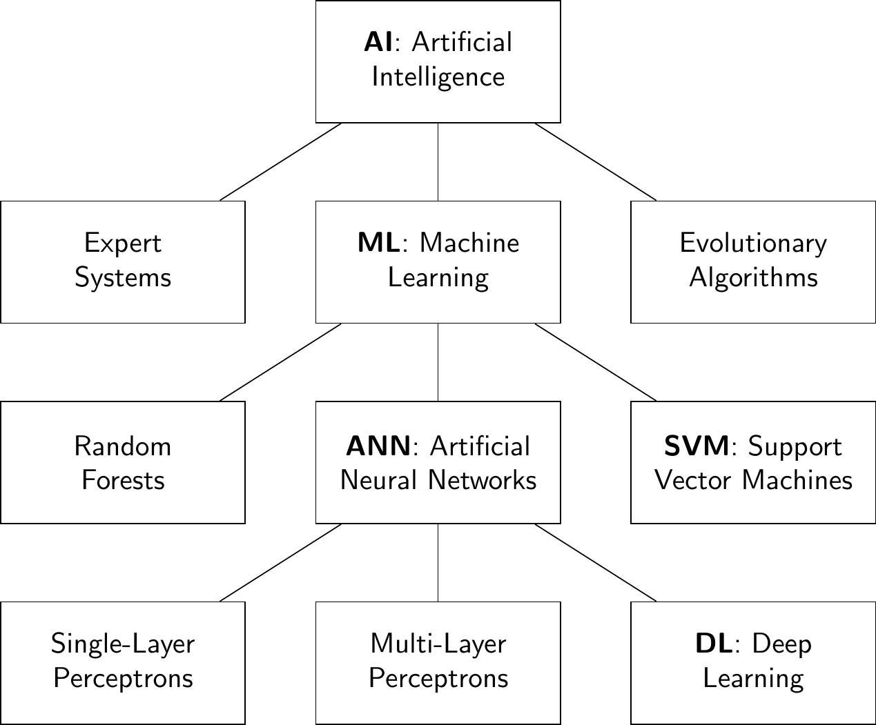
Figure 2.1: Hierarchical representation of AI and its sub-categories. This is non-exhaustive and is mainly intended to illustrate the place of deep learning within it.
2.2 Machine learning
Machine learning (ML) is a subfield of AI, aiming to create systems which are able to learn from data. Typically, an ML model is trained by iterating over data, updating the model’s parameters in order to gradually improve its accuracy on a given task. We distinguish between supervised and unsupervised learning. In supervised learning, the aim is to learn a mapping from input data to output data, where both are supplied to the algorithm. The desired outputs are referred to as labels. A popular example of a supervised learning task is, given a picture of either a cat or a dog, output the label ‘cat’ if the picture contains a cat, otherwise output the label ‘dog’. Note that a label does not need to be text, it could also be a numerical value, or a picture, or of any other data type.
In unsupervised learning, no labels are available. The goal in unsupervised learning is often to produce a simplified description of the data. The canonical example is that of clustering: dividing the input datapoints into a certain number of groups, such that points within a group are more similar than points across groups. When the goal is to learn the internal structure of the data (such as next word prediction in text, as done by large language models), it is often called self-supervised learning because the labels are given by the data itself. An intermediate category of ML between supervised and unsupervised learning is referred to as semi-supervised learning, where we wish to learn a mapping from inputs to outputs; however, only a fraction of the inputs is labeled.
Mathematically, a supervised learning model can be described as:
\[\begin{equation} \hat{y} = f \left( x, \theta \right) \end{equation}\]The term model refers both to the function \(f\) and to the parameters \(\theta.\) We provide input data \(x\) (e.g. the pixels of an image) and obtain the model’s predicted output \(\hat{y}\) (e.g. the label ‘cat’). The model learns to produce good predictions, by being shown many pairs of examples \((x,y)\) of input with true output. Often, the function \(f\) is fixed, and the training consists in finding values for \(\theta\) such that predictions \(\hat{y}\) are as close as possible to the given labels \(y,\) also called ground truth. For simple models, such as in linear or logistic regression, the best values for \(\theta\) can be found using a single, closed-form expression. For more complex models, iterative algorithms are usually employed, which are generally not guaranteed to converge to an optimal solution.
2.3 Training data
In machine learning, the data is typically split into disjoint subsets, called training set and test set. Often, there is also a third subset, called validation set. The training set is used to fit the model, that is, the model is allowed to ‘see’ the training data in full. The optional validation set can be used to assess when to stop training the model, or to select one among several competing models. The final model’s performance5 is then estimated by applying it to the unseen test set.
A short note on the word data: although data is originally the plural of datum (which is defined as a piece of information), most of the ML literature uses data as a singular noun, and this book follows the same convention.
2.4 Stochastic gradient descent (SGD)
The most commonly used algorithm in machine learning is stochastic gradient descent (SGD). It proceeds by computing the gradient of the loss function (to be minimized) at each optimization step, not unlike Newton’s method. The loss function measures6 the difference between predicted outputs \(\hat{y}\) and true labels \(y.\) The parameters are slightly modified in the direction of the gradient, in order to slightly improve the accuracy of the model. The ‘descent’ part of the name indicates that we follow the gradient downwards, continually decreasing the loss/error. The word ‘stochastic’ refers to the fact that we only use part of the data at each step of the algorithm, a small batch of randomly chosen data points. While gradient-based methods can be applied to a large class of models, in the case of neural networks, gradients are calculated using an efficient method called backpropagation, which implements the chain rule for differentiation. There exist several variations of SGD, called RMSProp [9], AdaGrad [10], Adam [11], etc. Gradients can be calculated automatically for nearly any given program, for example using the Autograd [12] reverse automatic differentiation system for the Python programming language.
2.5 Overfitting
In ML, we fit a model to data, using an algorithm such as SGD. In the supervised learning setting, this means that we search for parameter values \(\theta\) such that the predicted outputs \(\hat{y}\) are as close as possible to the true labels \(y\) given by the data. In this process, we can end up in the situation of overfitting, that is, we may find parameter values which are too closely molded to our particular dataset, which can happen if the function \(f\) has many degrees of freedom compared to the complexity of the data. This is illustrated in Figure 2.2, where three models (three different functions \(f\)) are fitted to the same data. In the leftmost panel, the model has too few degrees of freedom to capture the shape of the data, which is an underfitting situation. In the rightmost panel, we see the overfitting situation; the model is powerful enough to capture the shape of the data, but has in addition overzealously fitted small fluctuations that are likely due to sampling noise. The middle panel depicts a proper fit, which is the desired outcome in any ML application. Of course, in general, a visual inspection of the fit is not feasible, especially when the dataset is very large and/or high-dimensional. How, then, does one detect when a model overfits? This can be achieved by observing how accurate the model is on a validation set, which is a part of the dataset that has been withheld from the training set, i.e. which was not used to train the model (cf. Section 2.3). When the model keeps getting more accurate on the training set, but starts getting increasingly worse on the validation set, it is a sign that the model has begun to overfit.
There are several techniques to avoid overfitting. The obvious solution would be to simply choose a function \(f\) that is appropriate for the complexity of the dataset. However, this is a very difficult thing to do in general, beyond simple situations. Several practical techniques are described in this document.
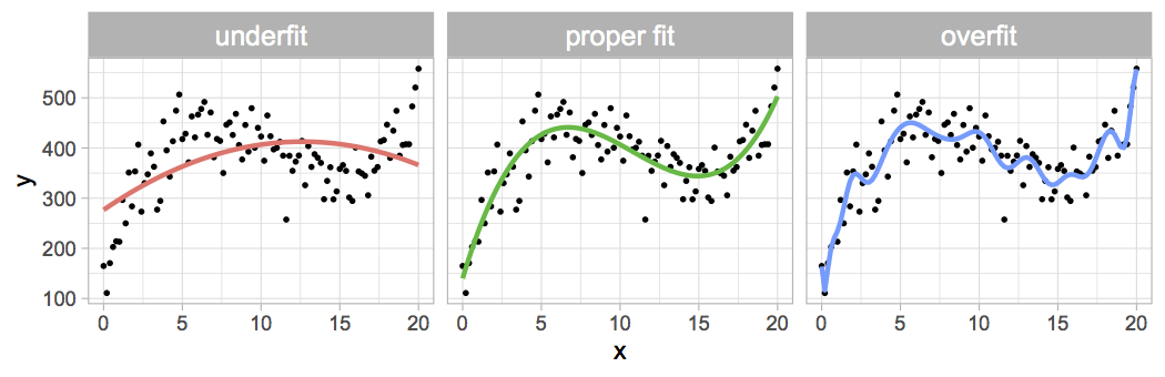
Figure 2.2: Illustration of the concept of overfitting. A given dataset of \((x,y)\) points, shown as black dots, is fit with three models of increasing expressive power. Left: underfitting situation, the model is not expressive enough to capture the data’s main shape. Middle: proper fit. Right: overfitting situation, the model attempts to capture minutiae of the dataset which are likely due to sampling noise.
2.6 Regularization
A common technique to avoid overfitting is called regularization. It consists in adding a term to the loss function, to represent the degrees of freedom used by the model’s parameters. Loosely speaking, the resulting loss function penalizes the model if it uses too many degrees of freedom, following the principle of Occam’s razor7. This technique is broadly applicable because it makes no strong assumptions about the type of ML model being used; however, it can be difficult to select a good functional form and weighting of the regularization term.
2.7 Artificial neural network (ANN)
An artificial neural network (ANN), often just called neural network, is a very commonly used ML model. Its design is inspired by biological neurons, which are connected together, and get triggered if their inputs are sufficiently active. Mathematically, an artificial neuron is composed of just two things: 1) a linear combination of inputs, and 2) a non-linear function applied to this sum. This corresponds to the following expression:
\[\begin{equation} output = activation \left( \theta_0 + \sum_{i=1}^P \theta_i \times input_i \right) \end{equation}\]where the neuron receives a fixed number of inputs, and associates with each \(input_i\) a parameter (or weight) \(\theta_i.\) Note that a neuron’s input can come directly from data (e.g. a pixel value) or from the output of another neuron. The term \(\theta_0\) is referred to as the bias of the neuron.
The activation function is a non-linear function. Historically, the sigmoid and tanh functions were predominantly used, but presently, piecewise linear functions such as the rectified linear unit (ReLU) [13], [14] are the most common, cf. Figure 2.3.
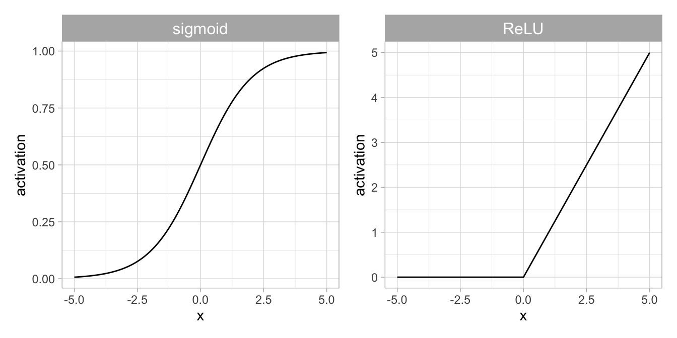
Figure 2.3: Non-linear activation functions commonly used in artificial neural networks. Left: Sigmoid function. Right: Rectified Linear Unit (\(ReLU\)).
2.8 Deep learning (DL)
In a neural network, multiple neurons are connected together, the outputs of one neuron being fed as input into others. Neurons can be arranged in layers, such that the input data gets fed into the first layer, the outputs of which get fed into the second layer, and so on, and the model output is provided by the final layer. The term deep learning (DL) refers to ANNs consisting of many layers. Such models were originally difficult to train efficiently, but the increased computational power of GPUs and ASICs, as well as algorithmic improvements, has made DL practical since the early 2010s; GPUs are extremely well suited to perform computations on matrices and tensors8 (more on this in Chapter 5). The depth of the model is increased to enable the handling of complex data. For example, in the context of image data, the layers are able to represent concepts of increasing hierarchical aggregation. The first layer might capture basic concepts like edges and contrasts, the second layer might combine those concepts to capture simple shapes. These are in turn combined into more complex shapes, until finally in later layers, the neurons are able to detect a cat, or a dog. Such high-level ‘features’, such as cat or dog, emerge by themselves, simply by training a deep learning model. Previously, features were largely handcrafted in a labor-intensive process known as feature engineering, but deep learning has automated this and made it much more efficient.
The architecture of a DL model refers to the types of neural layers used in the model, and to the topology in which they are interconnected. Below we list several common architectures, such as the CNN and the transformer.
2.9 Dropout
Dropout is an important overfitting avoidance technique in DL. It consists in disabling a random subset of the neurons during each training step. This forces the model to build in robustness and redundancy, and drastically reduces overfitting, even in models with an immense number of parameters (at the time of writing, the size of the largest models is crossing the trillion parameter mark [15], and the trend is towards ever bigger models).
2.10 Convolutional neural network (CNN)
One of the most common DL architectures is the convolutional neural network. The term refers to a specific way in which neurons in one layer are connected to neurons in the subsequent layer(s) of the network. The simplest architecture is called fully connected: the output of every neuron in layer \(k\) is connected to the input of every neuron in layer \(k+1.\) The fully connected approach results in a very large number of parameters, and does not make use of the fact that pixels which are close to each other are more likely to be related. By contrast, in a CNN, a neuron in layer \(k+1\) receives as input only a small ‘window’ of pixels from layer \(k.\) In addition, the weights are the same for each window, which is referred to as weight sharing. These two architectures are compared in Figure 2.4. The convolutional concept can also be extended to higher dimensions; in fact, the most common application of CNNs has been to process 2D images since their inception [16], [17], cf. Figures 2.5 and 2.6. There are many variations of convolution, including the addition of padding around the input in order to obtain an equally sized output, or only applying the filter at each \(n\)-th position of the input (\(n\) is then called the stride), etc.
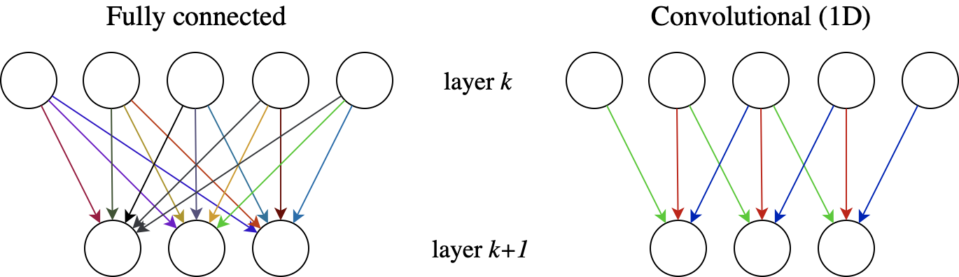
Figure 2.4: Two neural network architectures. Left: fully connected. Every neuron in layer \(k\) feeds into every neuron in layer \(k+1,\) and each connection has its own specific weight parameter, represented by the variety of colors. Right: convolutional (1D). Each neuron in layer \(k+1\) receives input only from a small neighborhood of neurons in layer k. Moreover, the incoming set of weights is identical for each neuron in layer \(k+1.\)
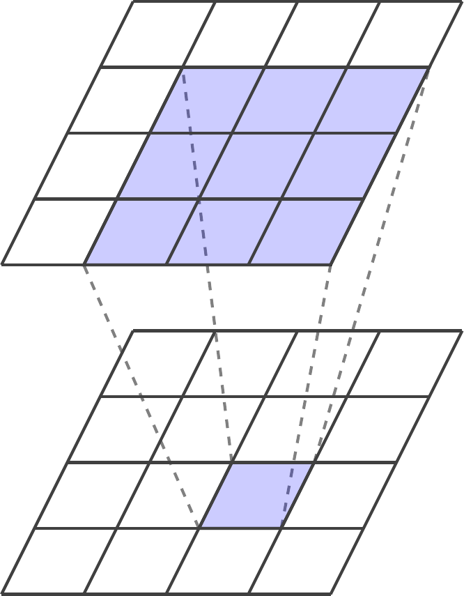
Figure 2.5: Simplified illustration of a single two-dimensional convolutional layer of depth one. The value of an element in the output tensor is computed based on a small neighborhood of elements in the input tensor, here using a window of size \(3 \times 3.\) A convolutional layer typically contains many filters and the input tensor can be of arbitrary depth, as shown in Figure 2.6.
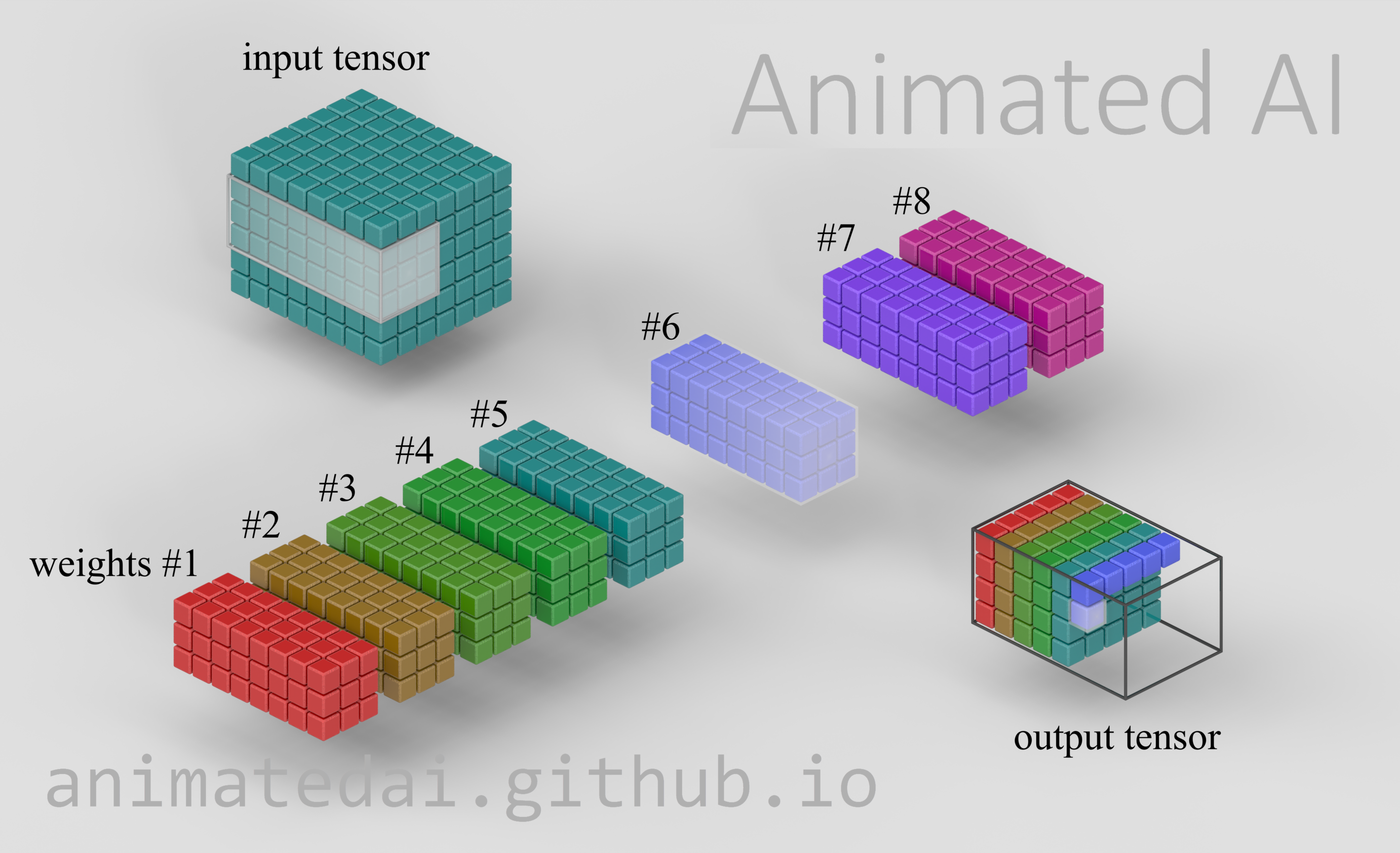
Figure 2.6: Illustration of the full computation performed by a 2D convolutional layer. This layer has eight sets of weights (also referred to as eight filters), numbered 1 to 8. The filters are size \(3 \times 3\) and they have the same depth as the input tensor. Each filter is used in turn, in combination with the input tensor, to compute a slice of the output tensor, as indicated by the colors. This image is a frame taken from an animation, after filters 1 to 5 have already been applied, and filter 6 is being processed. At this moment, the filter is being multiplied by the highlighted section of the input tensor, and the nonlinearly transformed sum of this calculation is stored in the highlighted element of the output tensor. Once completed, the output tensor will have depth 8, the same as the number of filters. The full animation, along with other excellent deep learning animations created by Brad Klingensmith, can be viewed at .
2.11 Recurrent neural network (RNN)
Typically, neural networks are connected in a feed-forward topology, one layer being connected to the next, without ‘loops’ returning to a previous layer. Networks which contain such loops are called recurrent neural networks. Such networks are much more difficult to train than the feed-forward kind, since the loops can lead to numerical challenges in the learning process. Large gradients get even more amplified, while small gradients quickly go to zero, both of which impede a smooth gradient descent process. Despite this challenge, RNNs have seen significant research interest, because of their capability to handle variable-length inputs and outputs, as is the case for example in text translation from one language to another; sentences can be of any length, and the length of a French sentence is often not the same as that of its English equivalent. This class of learning problems is often referred to as sequence-to-sequence problems. recurrent neural networks using designs such as Long Short-Term Memory (LSTM) were the most successful ML models for these tasks for several years, but they have largely been displaced by alternative architectures such as the transformer models.
2.12 Transformer
The term transformer refers to a neural network architecture that has become highly prevalent in the past few years. Transformers were invented in the context of sequence-to-sequence problems such as text translation [18]. In particular, they are designed to overcome the limited training efficiency of RNNs (they can make much better use of GPUs than RNNs can). However, transformers are not limited to textual data, but are also applicable to image processing (vision transformers (ViT)) [19], and in fact they turn out to be strong competitors to the CNN models which have been dominating that space for a decade. The mechanism at the heart of transformers is called attention, for it mimics the human ability to temporarily focus one’s attention to some specific thing while ignoring others. In particular, it allows the model to fetch the pieces of information that provide the most relevant context to the particular processing step being performed, even if that information is not in the immediate vicinity of each other. In a typical English sentence, one or a few words carry most of the important meaning, while the rest of the words act as support and are much more predictable. Since the real information content is concentrated in a few select locations, rather than uniformly spread out over the entire sentence, it makes sense to pay particular attention to those important locations, and the transformer integrates several such ‘attention heads’ in its design.
2.13 Reinforcement learning (RL)
Reinforcement learning (RL) is an area of machine learning where we wish to learn a function based on data that is only sparsely labeled. Typically, the objective is to learn an agent strategy involving a possibly long and complex sequence of actions, to achieve a certain outcome. For example, think of a game of chess, wherein one moves many pieces, in response to the moves of one’s opponent, until ultimately arriving at the game’s conclusion (win/loss/draw). Learning exactly which combination of actions – or avoidance of actions – led to a certain outcome, can be very difficult. A similar challenge arises when designing the control system of a robot with many degrees of freedom, to perform tasks in a complex environment. Reinforcement learning is the study of ML approaches in settings such as these, and has been in the popular spotlight since the company DeepMind used it in combination with deep learning, in a series of highly successful game-playing algorithms, such as AlphaGo and AlphaZero, which are able defeat the world’s best human players in the game of Go. The word ‘reinforcement’ is borrowed from psychology, where positive reinforcement refers to the rewarding of good behavior, such as giving a treat to a dog for obeying a command. This same principle is applied to learning a good strategy.
RL has been applied to large language models (LLMs) in order to make them more conversational or otherwise appropriate. A model that was previously trained on an enormous body of text in an unsupervised fashion, is then fine-tuned using painstaking human annotations or scoring for some of its raw outputs. In this context, the technique is referred to as reinforcement learning from human feedback (RLHF) [20].
2.14 Generative model
A generative model is a statistical or ML model that approximates the joint probability distribution \(P(x,y)\) of inputs and outputs (or simply the probability distribution \(P(x)\) of inputs), rather than the conditional probability \(P(y|x)\) of output given the input. In the latter case, the model is usually called a discriminative model. Once trained, a discriminative model is able to tell us whether there is a bird in a given input picture, whereas a generative model can allow us to sample from the input distribution, in other words, to generate a (previously unseen) bird. There are several approaches to creating generative models, including Generative Adversarial Networks (GANs), Variational Auto-Encoders (VAEs), diffusion models, etc. Generative models are a fast-evolving area of research and development, and Chapter 7 is dedicated to discussing their current state of the art and frontiers.
2.15 Diffusion model
A diffusion model is a generative model that is trained to progressively ‘de-noise’ a noisy image [21]. In this approach, it is very easy to obtain copious amounts of training data, by simply taking a high-quality image and gradually adding noise to it, cf. the sequence of images in Figure 2.7, from left to right. The model is trained to achieve the transformation in the opposite direction, i.e. from right to left. Ultimately, when the model becomes proficient at this task, we are able to inject a purely random signal, from which the model generates a plausible exemplar of the input distribution (e.g. a bird). This process can take place in pixel space, as in the illustration, or it can take place in a more abstract space. A popular approach of the latter idea is called latent diffusion [22], where the diffusion is performed in a low-dimensional latent space, allowing for more efficient learning.
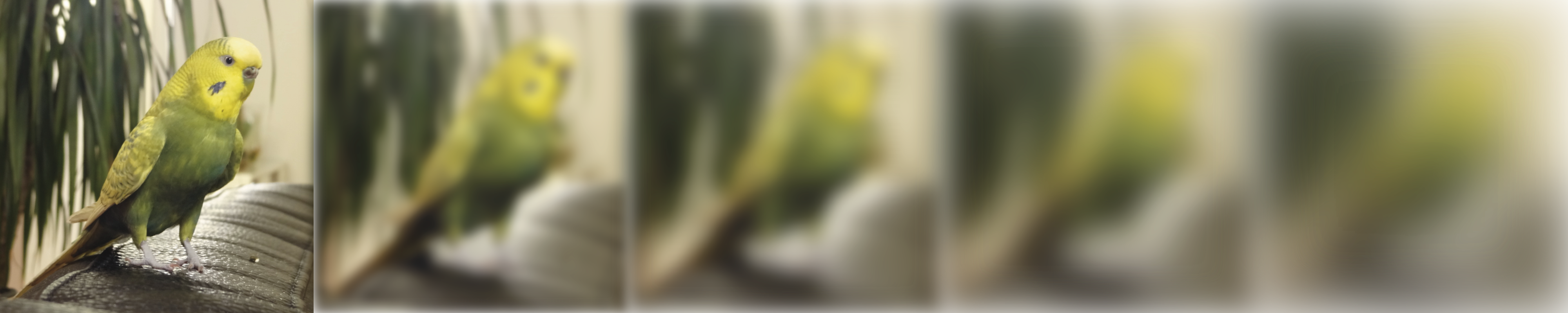
Figure 2.7: Diffusion model illustration. An image is put through successive additions of noise (left to right). The ML model is trained to restore the image, which amounts to ‘undoing’ the noise addition. Such a model is then able to generate images from pure noise.
2.16 Transfer learning
Transfer learning is a widely applied method in deep learning. It consists in repurposing a model for a different task than the one that it was trained for. This capability of DL came as a surprise in the field of machine learning, where beforehand, a model trained for one purpose was considered to be largely unusable for another, in most cases.
Training a large model from scratch can require extensive computational resources and infrastructure, and transfer learning enables the economizing of such resources, by leveraging prior training in a new context. Another important motivation for transfer learning is that there may not be a large labeled dataset available for learning the new task, and using a pretrained model can strongly reduce the data requirements. Typically, only a few layers of the deep neural network are significantly modified, while leaving the other layers largely unchanged. Adapting a model to a new task in this way is referred to as fine-tuning in the literature.
2.17 Causal model
All scientists are familiar with the adage, ‘correlation does not imply causation’. We cannot establish a causal relationship between two variables merely based on an observed statistical association (e.g. correlation) between them. All of the machine learning techniques previously discussed in this chapter are based on statistical association. A causal model is a type of model that aims to capture causal relationships instead. They are beginning to be used to infer causation from time series data in Earth System Science [23]. Causal Models are a different branch of AI, and interested readers are referred to Pearl and Mackenzie [24] for a conceptual introduction, and to Peters et al. [25] for more technical depth. This topic will be expanded on in Chapter 8.