4 AI and challenges in Earth-related sciences
Many phenomena under study in the Earth-related sciences demonstrate aspects that we have come to describe as teleconnections, cross-talk, weak signals, non-linear dynamics, phase changes, and chaos. In this chapter, we outline how AI methods (in particular deep learning) are suitable for dealing with these issues.
4.1 Correlations/teleconnections
Deep learning is very effective at finding correlations in data, which can be harnessed to achieve high predictive power. Although correlations are easiest to discover when the spatial or temporal gap between the correlated signals is small, correlations can nevertheless be learned in the presence of large gaps as well, such as in the context of teleconnections, when predicting the regional water cycle based on the low-frequency climate modes of variability of El Niño Southern Oscillation (ENSO) [55]. While correlation does not equal causation, causation induces correlation, and detecting correlation can put scientists on the path of uncovering causal mechanisms. Increasingly, techniques are being developed which enable scientists to locate and characterize the underlying sources of correlation. Hence, while a ML model may not provide a causal explanation, it can be used to generate leads for investigating underlying physical causes. The correlation vs. causation question is examined in greater detail in Chapter 8. However, in the context of ENSO, saliency maps (Section 3.1) have been utilized to extract interpretable predictive signals from global sea surface temperature and to discover dependence structure that is relevant for quantitative prediction of river flows [56]. Machine learning has also been used to study relationships among teleconnections on a seasonal timescale, between the North Atlantic Oscillation, the Pacific North American Oscillation, the West Pacific Oscillation, and the Arctic Oscillation [57].
4.2 Cross-talk and weak signals
When multiple phenomena are coupled in their underlying physical, electro-magnetic, or chemical make-up, through a form of energy transfer, these phenomena can be considered to act as a single system. We refer to this energy transfer as cross-talk, and it can occur in many engineered and natural settings. Two electrical circuits which are in close proximity can exhibit cross-talk from radiative effects, as can wave trains in the ocean that emanate from separate storms when they come close and interact. In such situations, a common approach is to consider each phenomenon as a subsystem. These subsystems are then assembled into a larger system by explicitly linking them together through a mechanistic or otherwise well-known scheme. By contrast, the typical DL approach is to consider the entire dataset from the viewpoint of a single model, letting the learning process itself figure out the dynamics of the full system. Alternatively, outputs for individual subsystems can be provided alongside the full data, so that the DL network can self-select any useful signals. Such approaches are proving very effective in engineering, in particular for the removal of crosstalk where it is typically undesired [58],[59]. In natural settings, the focus is typically not on crosstalk removal; however, it remains important to understand when and where it occurs. In biology, crosstalk refers to the intercommunication between different signaling pathways or cellular processes, involving the transfer of signals or molecules from one pathway to another, with a possible effect on the overall cellular response. The resolution of biological data having in some cases gone down to the single cell level, deep learning has been applied in the analysis of the resulting large datasets, with promising results across many topics, including in single-cell genomics and transcriptomics [60]. The above applications may provide inspiration to Earth Science practitioners and could be translated to some ES contexts, in particular in Earth Systems Science.
In numerous scientific investigations, we are faced with weak signals, that is, signals which are largely or very nearly drowned out by noise, or are so sparse that they are difficult to measure. For instance, gravitational waves generated by black hole collisions, travelling across the cosmos, have only recently become measurable thanks to LIGO detectors. In addition to bespoke instruments, such weak signals may need special processing to become evident, which can take the form of ML and DL11 [62]. We may also refer to weak signals in the context of scientific modeling, such as when creating a mathematical model of a phenomenon where we have discarded higher-order terms as being negligible, in order to make the model more tractable and easier to study analytically. However, even if those terms are small in comparison to the dominant ones, they may drive a system behavior that turns out to be important, especially at different spatiotemporal scales. In particular as the system approaches a tipping point in its state of equilibrium, the interplay between small effects can result in a non-negligible difference in outcome. The compounding build-up of vorticity, turbulence and eddy currents from sub-micro level origins into large-scale behavior patterns within the Earth’s oceans and atmosphere is a commonly recognized process. Neural networks are showing promise for predicting ocean surface currents accurately, as compared to physical simulation models [63].
4.3 Non-linearity
As was mentioned earlier, the default preference in science lies with simpler models, all else being equal. Linear models are among the simplest, relating a dependent variable with one or more independent variables through a linear combination. One of the most ubiquitous statistical models of this kind is the linear regression,
\[\begin{equation} y_i = \beta_0 + \sum_{j=1}^p \beta_j x_{i,j} + \epsilon_i \end{equation}\]where \((x_i,y_i)\) is the \(i\)-th data point, \(x_i\) being a vector of size \(p.\) Furthermore, \(\beta_j\) is the \(j\)-th parameter of the model, and \(\epsilon_i\) are the noise terms, assumed to be independent identically distributed Gaussian random variables. This model is very popular, because its parameters lend themselves to a relatively straightforward interpretation, and because it has a single, closed form solution. Many natural phenomena involving numerous interacting and evolving processes on the other hand, cannot be modeled accurately using a linear model. The linear regression model can be generalized in various ways in order to deal with non-linear relationships; however, the aforementioned advantages decrease or disappear as models get more expressive, and choosing the correct type of model for a problem requires a high degree of expertise. In some such situations, deep learning can be a good alternative. Fitting a DL model to a large dataset is likely to require less domain knowledge and modeling proficiency than applying a tailored non-linear approach.
Differential equations constitute another very important scientific modeling tool, especially in the context of many Earth related disciplines. Here again, we need to ‘switch gears’ when non-linearity is introduced. Indeed, consider a dynamical system characterized by the equation,
\[\begin{equation} \dot{x} = f(x,t) \end{equation}\]where \(x\) is a vector, and the right-hand side is a vector field that depends on time \(t.\) If the function \(f\) is linear in \(x,\) the system is completely characterized by the eigenvalues of \(f.\) However, non-linearity in the function very often results in the absence of a closed-form solution, making the analysis, simulation or prediction concerning this system much more difficult. In many cases, in addition to being non-linear, \(f\) is effectively unknown, and machine learning can be a helpful tool to learn non-linear PDEs from data [64].
4.4 Feedback loops
In nature, we often encounter situations in which one phenomenon increases (or decreases) the frequency or intensity of another phenomenon. In many cases, this influence is bidirectional – the phenomena affect each other. We then speak of feedback loops. In particular, if each phenomenon has the effect of increasing the other in amplitude, the feedback is called positive or self-reinforcing. As an example, consider the arctic sea-ice melting from a warming ocean, decreasing the albedo of the planet, and causing the sea to absorb more energy from sunlight because of its darker color than if ice covered, thereby heating the upper ocean layers even higher, which in turn contributes to further sea-ice melting. Since feedback loops give rise to correlations, DL will be able to incorporate this signal for increased predictive power. However, a complex network of interacting positive and negative feedback loops may be difficult for a DL model to unravel, especially if it is not trained on a dataset which covers most possible states, or at least a sufficient selection of states such that interpolation between them leads to meaningful predictions. In the absence of sufficiently complete data, explicit modeling of domain knowledge is likely to be required, and in this regard the blending of neural networks with physics-informed partial differential equations can provide an answer [65].
4.5 Phase changes
The most familiar phase changes we encounter are those of water. When the temperature of water drops to zero degrees Celsius, it freezes; its state of matter changes from liquid to solid. Melting, vaporization and condensation are also phase changes – physical processes of transition between various states of matter, which occur when the pressure and temperature cross certain boundaries, as illustrated in Figure 4.1. More generally, we can think of a phase change as a qualitative shift in the basic structure and behavior of a system. Machine learning can be applied to identify when such shifts occur, which is especially useful when the physical parameters are not known in detail. Neural networks were used successfully for the classification of phase changes and states of matter in highly intricate settings, such as in quantum-mechanical systems [66]. Neural networks were also applied in combination with atomistic simulations and first-principles physics to generate phase diagrams for materials far from equilibrium [67]. Specifically, deep learning was used to learn the Gibbs free energy, and phase boundaries were determined using support vector machines (SVM). The obtained ‘metastable’ phase diagrams allowed the identification of relative stability and synthesizability of materials, and the phase predictions were experimentally confirmed in the case of carbon as a prototypical system. Phase diagrams are also of interest at much larger scales, such as in the context of the Earth’s climate. Consider for example the schematic phase diagram shown in Figure 2 of Lessons on Climate Sensitivity from Past Climate Changes [68], plotting the planet’s global mean surface temperature versus the atmospheric carbon dioxide concentration, featuring two disjoint branches: a ‘cold’ branch for a climate with polar ice sheets, and a ‘warm’ branch for a climate without them. Potentially, AI could assist in deriving such diagrams, but in more detail.

Figure 4.1: Phase diagram for water. When the system’s state crosses a boundary (solid green line), a phase change occurs.
4.6 Chaos
Many phenomena in nature exhibit chaotic behavior, making them very hard to predict. In a chaotic system, the outcome is highly sensitive to initial conditions, a property that is often referred to as the ‘butterfly effect’. A tiny change at the start of the process can lead to dramatically different final results. There is evidence that machine learning can be used to improve predictability even in such seemingly hopeless cases, as was demonstrated in the context of the Kuramoto-Sivashinsky equation, also called the ‘flame equation’ because it models the diffusive instabilities in a laminar flame front, a simulation of which is shown in Figure 4.2. A neural network model was trained to forecast the evolution of the system, without the model having access to the equation itself. The research team were able to achieve accurate predictions much further into the future than was previously thought possible [69], [70].
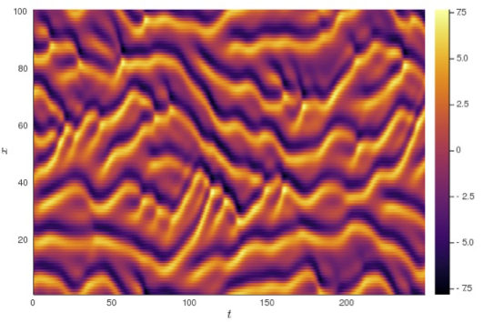
Figure 4.2: Plot of a simulation run of the Kuramoto-Sivashinsky flame equation. For each timestep on the horizontal axis, the flame front is described as a vertical strip of colors. Image credit: Eviatar Bach (Creative Commons CC0 1.0) using source code by Jonas Isensee.