8 Causal models: AI that asks ‘why’ and ‘what if’
As deep learning scales up at a steep exponential rate, in both industry and academia, another branch of AI is currently much less prevalent, yet it may be just as fruitful in the long run, if not more so. The paradigm goes under the umbrella term of causal models, and has been championed among others by Judea Pearl, who won the 2011 ACM Turing award for ‘fundamental contributions to artificial intelligence through the development of a calculus for probabilistic and causal reasoning’. This chapter describes some fundamental concepts of causal models, and highlights some of its uses in studying Earth systems.
8.1 Causation vs correlation
The fundamental distinction between standard machine learning and causal modeling is that the former is based on correlation, while the latter focuses on causes and effects. Correlation refers to a statistical association between two variables, and students worldwide are taught that correlation does not imply causation. When we notice that two variables \(X\) and \(Y\) move in tandem, we know that this may be due to a number of reasons. It could be that \(X\) has a causal effect on \(Y.\) It could also be that \(Y\) has a causal effect on \(X.\) Likewise, it may be that a common cause \(W\) has a causal effect on both \(X\) and \(Y.\) In this case, \(W\) is often called a confounder. More subtly, it could be that the dataset under study has a selection bias, which can arise when its datapoints are selected according to a common effect \(Z\) of \(X\) and \(Y.\) Such a selection bias can distort the statistical relationship between \(X\) and \(Y.\) For example, if we wished to analyze the causal effect of sprint training on leg muscle mass, then using a dataset containing only Olympic sprinters would be a poor choice; that dataset has a strong selection bias, as it focuses on the individuals with the world’s very fastest running speeds, and running speed is causally influenced by both sprint training and leg muscle mass.
This is an example of what is referred to as a spurious correlation in the causality literature: a statistical association between variables that does not coincide with the causal relationship between these variables. Note that a correlation could also be accidental, which is popularly referred to as a spurious correlation as well, although its meaning differs from the one outlined above. An example of such a correlation is the one observed between the volume of Google searches for ‘zombie’ and the number of real estate agents in North Dakota, for the years 2004-2022, shown in Figure 8.1. This correlation would very likely disappear if we used a larger dataset. In the rest of this chapter, we will assume that sample sizes are large, in order to focus on the main concepts of causal models. However, it should be kept in mind that any limitations of classical statistical methods, when used on small samples, would also apply in the case of causal models.
![Example of a spurious correlation in the ‘accidental’ sense. The relative volume of Google searches for ‘zombies’ is highly correlated with the number of real estate agents in North Dakota (data sources: Google Trends, US Bureau of Labor Statistics), with an \(r\) value of 0.936. This correlation, and a sizeable collection of others like it, were obtained by data dredging a large database of time series: testing many possible pairwise combinations of time series, over many time segments and intervals. When one does this without adjusting the threshold for statistical significance (e.g. using the Bonferroni correction [134], [135]), many false positives can result. This is also referred to as p-hacking in some contexts. The collection of humorous correlations is curated by Tyler Vigen at .](images/spurious_vigen/spurious_zombies_realestate.svg)
Figure 8.1: Example of a spurious correlation in the ‘accidental’ sense. The relative volume of Google searches for ‘zombies’ is highly correlated with the number of real estate agents in North Dakota (data sources: Google Trends, US Bureau of Labor Statistics), with an \(r\) value of 0.936. This correlation, and a sizeable collection of others like it, were obtained by data dredging a large database of time series: testing many possible pairwise combinations of time series, over many time segments and intervals. When one does this without adjusting the threshold for statistical significance (e.g. using the Bonferroni correction [134], [135]), many false positives can result. This is also referred to as p-hacking in some contexts. The collection of humorous correlations is curated by Tyler Vigen at .
Many researchers argue that standard machine learning models learn the statistical patterns present in the data, but do not have a concept of the causal underpinnings that gave rise to the data. Due to their black box design and large size, it is difficult to check whether deep learning models build internal representations of causal concepts or not. For example, large language models do manifest some level of apparent causal reasoning ability. However, they are still comparatively weak at such reasoning tasks, so it is plausible that the bit of causal reasoning they do exhibit, simply mimics similar or analogous text in the training data. Indeed, as was previously mentioned, there are reasons to suspect that they are just ‘causal parrots’ [132]. Causal models, on the other hand, are built on a completely different premise. They are explicitly designed to incorporate causal knowledge and assumptions, and to answer causal questions.
8.2 Causal graphs
Causal methods were developed within multiple different disciplines, from econometrics to epidemiology to computer science, and therefore they come in many variations. One practice that has found widespread adoption is the use of causal graphs23, also referred to as causal diagrams. A causal graph is a graph in which nodes represent variables, and edges represent causal influences. If there is an edge from node \(X\) to node \(Y,\) it signifies that \(X\) causally affects \(Y,\) in the sense that if we were to surgically change \(X,\) then \(Y\) would change in response. Pearl describes this by stating that ‘\(Y\) listens to \(X\)’ [24]. For example, consider the causal graph in Figure 8.2. It describes causal relationships between the insolation \(I\) a tree receives from the sun, the tree’s growth \(G,\) and the presence of clouds \(C.\) Specifically, it posits that insolation causally affects growth, and that clouds causally affect insolation.
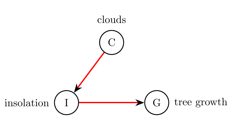
Figure 8.2: Example of a causal graph. According to this graph, insolation \(I\) has a causal effect on tree growth \(G,\) and clouds \(C\) have a causal effect on \(I.\)
The graph can be used as a means to communicate a hypothesis, which is readily understood by humans, and can serve to make questions and assumptions explicit. For instance, a colleague may point out that in order to model the situation more accurately, a direct edge from \(C\) to \(G\) is also needed, because sufficient water is necessary for tree growth, and clouds are necessary for rain. In other words, they may propose the causal graph in Figure 8.3 as an alternative hypothesis. Of course, one could add more variables, such as rain and soil moisture, in order to provide a causal description that is appropriate for the research question at hand, especially if data for these variables is also available.
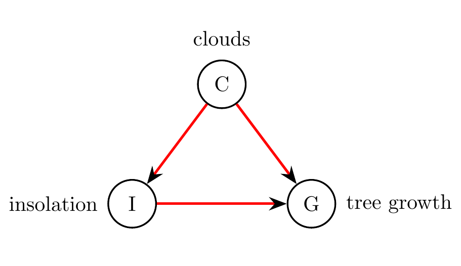
Figure 8.3: Alternative causal graph to Figure 8.2, in which a direct edge from clouds \(C\) to tree growth \(G\) is added, in order to model the effect of rain.
8.3 Causal inference
In addition to being human-readable, a causal graph is also machine-readable. It can be provided as a hypothesis to a causal inference engine, together with data. The engine is then able to check whether the graph is plausible with respect to the data, or whether the graph must be rejected. Furthermore, the engine can use the data and the graph to fit a quantitative model, which can then be used to answer queries about the system. In this instance, an example query could be, ‘if we decrease insolation by 10%, what change will we see in tree growth?’ An important point here is that this query can in general not be answered simply by looking at the conditional distribution of tree growth given insolation. There is a key difference between \(G\) given that we observe \(I,\) and \(G\) given that we impose \(I\) (i.e., that we intervene so as to force \(I\) to take on a certain value or distribution). For instance, suppose we intervened on insolation \(I\) in Figure 8.3, by blocking off the sunlight to the tree with a large screen or wall, and shining a large electric light on the tree, with an equivalent light spectrum, but using an intensity of our choosing. With this setup, we could now set the intensity so that it ‘replays’ the insolation observed during the previous week. The tree growth occurring with this chosen artificial insolation may be quite different from the tree growth that was observed for the previous week, because the causal effect of clouds on tree growth still remains, and we have not intervened on this variable \(C.\) Effectively, by intervening on insolation \(I,\) we transform the causal graph into what is shown in Figure 8.4, where the edge from clouds to insolation has been removed. Indeed, we’ve severed this causal influence, freely choosing the insolation.
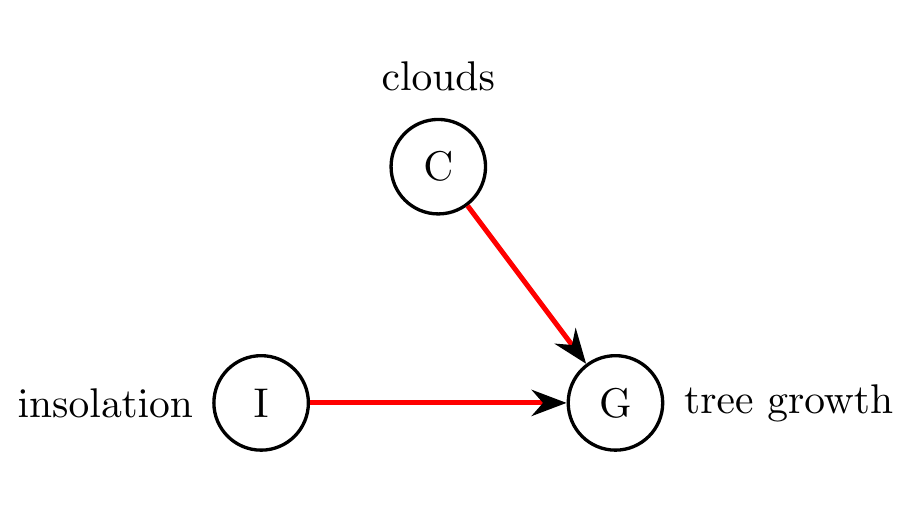
Figure 8.4: Modified causal graph from Figure 8.3, where we’ve intervened on insolation \(I.\) Since there is no longer a causal influence of clouds on insolation, the edge from \(C\) to \(I\) is removed.
The do-calculus is an important mathematical formalism for handling the distinction between observational and interventional probabilities. Its key innovation is the addition of the do-operator, which allows one to express an intervention. For example, \(do(I=i)\) corresponds to the intervention of setting insolation \(I\) to the value \(i.\) The expected value of tree growth \(G\) under this intervention can be written as \(E[G|do(I=i)],\) and as discussed, it is not the same as \(E[G|I=i]\) in general. The do-calculus provides a complete set of rules for converting between causal quantities and statistical quantities. For example, based on the graph in Figure 8.3, the statistical quantity obtained through do-calculus is the following24:
\[\begin{equation} E[G|do(I = i)] = E_C[E[G|I=i,C]]. \end{equation}\]Remarkably, in this case, we are able to answer a causal query using only observational data. If we have good reason to believe that the causal graph is correct, then we need not perform an experiment requiring the expenses of a large wall and a gigantic floodlight. Of course, the result is only as valid as the causal assumptions.
8.4 Assumptions and limitations
Assumptions are a cornerstone of causal inference. Some of these assumptions are testable, others are not. For instance, assumptions in the form of a causal graph are usually testable, if appropriate observational or experimental/interventional datasets are provided. Other assumptions can be difficult or impossible to test. For example, an assumption that is frequently made in causal inference is that there are no hidden confounders, i.e. that the causal graph captures all variables that are causally relevant to the question being posed, also known as the causal sufficiency assumption. Another common assumption is that there is a one-to-one correspondence between the causal graph’s structure and the conditional independencies that exist in the joint distribution over all its variables (technically called the Markov and faithfulness assumptions). The stronger the assumptions, the further the inference engine can leap, but the more justification needs to be supplied as to why the assumptions are reasonable in the context of what is being modeled. In this sense, there is a tradeoff between the strength of the assumptions, and the believability of the conclusions.
In many causal methods, one assumes that the causal graph is acyclic, i.e. contains no directed cycles, in the sense that walking the graph from node to node along the edges, in the direction of the arrows, never leads to revisiting a previously visited node. This seems like a strong limitation in the context of Earth systems, where feedback loops abound (cf. Section 4.4). However, methods for the causal analysis of time series can deal with this by using time indices for each relevant variable. See for example Figure 8.5, where a simple feedback loop between two variables \(X\) and \(Y\) is depicted. Even though the graph itself contains no cycles, it is able to represent a mutual causal dependence between \(X\) and \(Y\) across time.
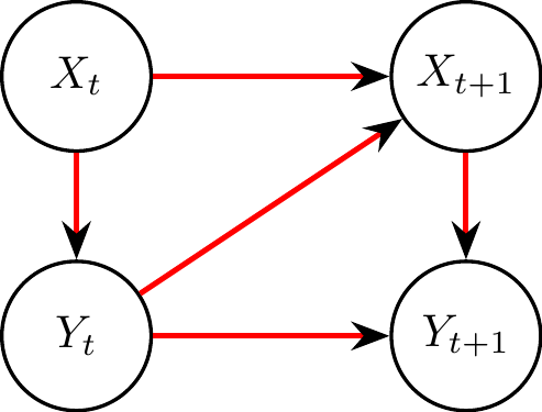
Figure 8.5: Causal graph containing a feedback loop between \(X\) and \(Y,\) even though the graph is acyclic. \(X_t\) represents the value of \(X\) at discrete time \(t,\) and equivalently for \(Y_t\) and \(Y.\) In this example, there is an instantaneous causal effect of \(X_t\) on \(Y_t,\) and a lagged causal effect from \(Y_t\) on \(X_{t+1}.\) Here each variable also causally influences its own future value.
8.5 Causal discovery
A part of causal research is aimed at ‘causal discovery’: ferreting out the causal graph from data. This can require a lot of data, and it is not always possible to obtain the full graph. For instance, causal discovery methods that are based on detecting conditional independence can only discover a set of graphs, called a Markov equivalence class, which in some cases could contain just a single graph, and in other cases contain multiple possible graphs that disagree on the direction of some of the edges. Many discovery methods are also unable to detect some subtle types of dependence. For example, if variables \(X,\) \(Y\) and \(Z\) are statistically dependent on each other, however they are pairwise independent (that is, \(X\) is independent of \(Y,\) \(X\) is independent of \(Z,\) and \(Y\) is independent of \(Z\))25, then most methods would prematurely and incorrectly conclude that there is no causal link between \(X,\) \(Y\) and \(Z.\) Of course, if we are able to obtain interventional data, e.g. by performing an experiment that intervenes on some of the system’s variables, our possibilities of causal discovery are increased.
As discussed in the previous section, making additional assumptions allows for more powerful causal inference, as long as those assumptions are justified. This also applies to causal discovery, where assumptions about the functional form of dependendance between the variables, as well as about the statistical distributions of noise, are very helpful. The linear Gaussian setting is the worst case for causal discovery, which may come as a surprise, since it is one of the simplest cases from a statistical modeling perspective. However, non-linear causal relationships between variables are often easier to detect than linear ones, as the non-linearities allow more aspects of the data-generating mechanisms to be identified [138]. Similarly, in a linear setting, if we have good reason to assume that the noise distributions are non-Gaussian, then causal discovery can be achieved where it is otherwise not feasible, e.g. using a linear non-Gaussian acyclic model (LiNGAM) [139]. Causal discovery is seeing an increasing number of applications in the Earth sciences, for instance in analyzing climatological time series. In particular, applying the PCMCI causal discovery algorithm [140] to surface pressure anomalies in the West Pacific and to surface air temperature anomalies in the Central Pacific and East Pacific yields a causal graph that identifies the well understood Walker circulation. A similar technique used for the Arctic climate detects that Barents and Kara sea ice concentrations are important drivers of mid-latitude circulation, influencing the winter Arctic Oscillation through multiple causal pathways. Readers are referred to Runge et al [23] for a comparison of several causal discovery approaches for time series in Earth Systems Science.
8.6 Interactions with machine learning and deep learning
For the time being, there is only limited interaction between causal research and the mainstream machine learning efforts focused on deep learning. For example, at Nvidia’s GTC conference in March 2024, out of a total of 337 online sessions, 261 matched the search term ‘AI’, and 130 matched ‘generative’, whereas searching for ‘causal’, ‘caused’ and ‘causality’ yielded one, one and zero results, respectively. Although causal models and deep learning are often not straightforward to combine26, achieving a synergy between the two would be highly valuable. They are somewhat akin to Kahneman’s fast and slow modes of thought [142]. Deep learning resembles our fast and instinctive ‘System 1’, with its remarkable abilities, but also replete with faulty shortcuts and biases. Causal models are closer to the slow and methodical ‘System 2’, using logic and careful deliberation based on facts and hypotheses. The combination of ‘System 1’ and ‘System 2’ is inarguably very useful to us humans, and quite possibly, a fusion between deep learning and causal models would represent a significant advance in AI.
While the two approaches have not yet been assembled into a holistic framework, there are some efforts to use deep learning and other ML techniques for the purposes of causal inference, causal discovery and discovery of equations from data. For instance, a technique known as ‘double machine learning’ can be used to adjust for confounding [143]. In the context of the example in Figure 8.3, this would amount to using ML to learn to predict \(I\) from \(C,\) and separately to learn \(G\) from \(C.\) Finally, an additional ML model then learns to predict \((G - \hat{G})\) from \((I - \hat{I}),\) where \(\hat{G}\) and \(\hat{I}\) are the predicted values of \(G\) and \(I,\) respectively, obtained in the previous step. Combining these pieces allows us to remove the confounding effect of \(C,\) and therefore to obtain an unbiased estimate of the causal effect of \(I\) on \(G.\)
On the research front of discovering invariants and equations from data, an approach called symbolic regression is used to search a space of mathematical expressions in order to find an equation or formula that describes the data accurately. Deep learning and reinforcement learning in various forms can make this search more efficient. For example, a recurrent neural network can be used to generate the expressions, in a framework called deep symbolic regression [144]. This approach can be further optimized by ensuring that only physically meaningful expressions are evaluated, as guided by the physical units of the variables [145]. The subfield of discovering equations from data has received significant attention of late, and the interested reader is referred to a recent review article [146].